
Production Planning, Process Control & Inventory Management (Workload, Scheduling, MRP, Ordering Systems)
生産計画と工程・資材在庫管理(工数・日程・MRP・発注方式)
Production Management Planning Grade 3 生産管理プランニング (BC検定) · ビジネス・キャリア検定 生産管理プランニング3級 · Written by Tokutei Pass based on the official study texts; not copied verbatim.
1. 工程管理の全体体系(生産計画の3分野と生産統制の5分野・使用帳票)
1. Overall System of Process Control (3 Areas of Production Planning, 5 Areas of Production Control, and Forms)
「工程管理」とは、定められた品質(Q)と原価(C)のもとで、顧客が要求する納期(D)と数量を確実に達成するため、仕事の流れと職場の生産能力を計画(Plan)・統制(Do・Check・Act)する活動です。
Process control is the activity of planning (Plan) and controlling (Do, Check, Act) work flow and shop-floor production capacity to reliably achieve the customer's required delivery date (D) and quantity under specified quality (Q) and cost (C).
計画機能である「生産計画」は3つの領域に分かれます。①加工順序や使用機械・方法を決める「手順計画」、②仕事量(負荷)と職場能力をバランスさせる「工数計画」、③いつからいつまでに造るかを決める「日程計画」です。
The planning function—Production Planning—is divided into three areas: (1) Process routing planning, which determines processing sequences, machines, and methods; (2) Workload (man-hour/capacity) planning, which balances workload and shop capacity; and (3) Scheduling, which determines start and completion dates.
実施と確認・処置を担う「生産統制」は5つの領域から成ります。①製造命令書や出庫票を発行する「作業手配」、②現場で作業の着手順序を指示する「ディスパッチング(差立て)」です。
The execution, check, and action function—Production Control—consists of five areas: (1) Order release / manufacturing preparation (issuing manufacturing orders and material requisition slips); and (2) Dispatching (directing the start order of jobs on the shop floor).
さらに③計画に対する遅れや進みを把握する「進捗管理(進度管理)」、④仕掛品の所在と数量を一致させる「現品管理」、⑤各職場の負荷と能力の過不足を調整する「余力管理」が加わります。
These are joined by (3) Progress control / expediting (tracking delays or advances against plan); (4) Physical inventory / WIP control (matching the physical location and quantity of work-in-process); and (5) Capacity / surplus power control (adjusting workload-capacity imbalances across shops).
Key points
- 生産計画の3分野:①手順計画(工程図・作業標準書)、②工数計画(負荷山積み表)、③日程計画(基準日程表・ガントチャート)。
Three areas of Production Planning: (1) Process routing planning (process charts, operation standards), (2) Workload planning (load accumulation charts), (3) Scheduling (master schedule tables, Gantt charts). - 生産統制の5分野:①手配(製造命令書・作業指導票・出庫票・移動票)、②ディスパッチング(差立て)、③進捗管理、④現品管理、⑤余力管理。
Five areas of Production Control: (1) Order release (manufacturing orders, job instruction tickets, issue slips, move tickets), (2) Dispatching, (3) Progress control, (4) Physical WIP control, (5) Surplus capacity control. - 手順計画は「どのように造るか」、工数計画は「どれだけの仕事量か」、日程計画は「いつ造るか」を決める。
Routing planning decides 'how to make', workload planning decides 'how much work volume', and scheduling decides 'when to make'.
| Word | Meaning |
|---|---|
| 生産計画(手順・工数・日程計画) | Production Planning (Routing, Workload, and Scheduling) |
| 生産統制(手配・差立て・進捗・現品・余力管理) | Production Control (Order release, Dispatching, Progress, Physical WIP, and Capacity control) |
| 製造命令書・作業指導票・出庫票・移動票 | Manufacturing order, Job instruction ticket, Material issue slip, Move ticket |
2. サプライチェーンマネジメント(SCM)と需要変動に対する3つの緩衝(モノ・能力・時間)
2. Supply Chain Management (SCM) and the 3 Buffers Against Demand Fluctuation (Inventory, Capacity, Time)
原材料や部品のサプライヤーから、製造工場、物流センター、卸売・小売店を経て最終消費者(顧客)に至るまでの「調達・生産・物流・販売」の連鎖全体を統合的に管理し、全体最適を図る手法を「サプライチェーンマネジメント(SCM)」と呼びます。
Integrally managing the entire chain of procurement, production, logistics, and sales—from raw material and parts suppliers through manufacturing plants, distribution centers, wholesalers, and retailers to final consumers—for total optimization is called Supply Chain Management (SCM).
サプライチェーン上で、需要予測に基づく「押出し(プッシュ型)生産」と、実需要(確定受注)に基づく「引張り(プル型)生産」が切り替わる境界点(戦略的に在庫を置く地点)が「デカップリングポイント」です。
Along the supply chain, the boundary point where forecast-driven push production switches to actual-demand-driven (confirmed order) pull production—and where strategic inventory is held—is the Decoupling Point.
市場の需要変動や予測誤差を吸収して安定供給を行うための「緩衝(バッファ)」には、「①モノによる緩衝」「②能力による緩衝」「③時間による緩衝」の3種類があります。
To absorb market demand fluctuations and forecast errors for stable supply, there are three types of buffers: (1) Buffer by goods (inventory), (2) Buffer by capacity, and (3) Buffer by time.
「①モノによる緩衝」は完成品や部品の安全在庫を持つこと(見込生産中心)、「②能力による緩衝」は残業・休日出勤・外注利用や予備設備で生産能力に余裕を持たせること、「③時間による緩衝」は顧客に待ってもらう納入リードタイム(納期余裕)で調整することです。
(1) Buffer by goods means holding safety stock of finished products or parts (central to Make-to-Stock); (2) Buffer by capacity means maintaining production capacity margin through overtime, holiday shifts, subcontracting, or standby equipment; and (3) Buffer by time means adjusting via delivery lead time waited by the customer.
Key points
- SCM=部品調達から生産・販売・顧客納入までの情報とモノの流れを一貫管理し、在庫削減とリードタイム短縮を図る手法。
SCM = End-to-end management of information and material flows from parts procurement to production, sales, and customer delivery to reduce inventory and shorten lead time. - 需要変動を吸収する3つの緩衝:①モノによる緩衝(製品・部品在庫)、②能力による緩衝(残業・外注・余剰設備)、③時間による緩衝(納期・リードタイムの調整)。
Three buffers absorbing demand fluctuations: (1) Goods buffer (product/parts inventory), (2) Capacity buffer (overtime, subcontracting, surplus equipment), (3) Time buffer (delivery date / lead-time adjustment). - 見込生産は「モノ(在庫)による緩衝」を主に使い、受注生産は「能力による緩衝」と「時間による緩衝」を主に使う。
Make-to-Stock primarily uses the goods (inventory) buffer, whereas Make-to-Order primarily uses the capacity buffer and time buffer.
| Word | Meaning |
|---|---|
| サプライチェーンマネジメント(SCM) | Supply Chain Management (SCM) |
| 3つの緩衝(モノの緩衝・能力の緩衝・時間の緩衝) | Three buffers (Goods buffer, Capacity buffer, Time buffer) |
| デカップリングポイントとブルウィップ効果 | Decoupling point and Bullwhip effect |
3. 生産計画の期間別階層(大・中・小日程計画)とローリング計画
3. Hierarchical Production Plans by Horizon (Master, Medium-, Short-Term Schedules) and Rolling Plans
生産計画は対象期間の長さにより階層的に立てられます。まず経営計画や販売計画を受けて、1年〜半年単位の品種グループ別生産枠や設備投資・人員計画を定める「長期生産計画(基本生産計画・大日程計画)」を作成します。
Production plans are established hierarchically by time horizon. First, based on business and sales plans, a Long-term production plan (basic production plan / master long-range schedule) is created in 1-year to 6-month units to set production quotas by product family, capital investment, and staffing plans.
次に3〜6か月または月次(1か月)単位で、製品別の月別生産数量と在庫水準・必要工数を定める「中期生産計画(総合生産計画・中日程計画)」、およびそれに基づく「基準生産計画(MPS)」を策定します。
Next, in 3-to-6-month or monthly (1-month) units, a Medium-term production plan (aggregate production plan / medium-range schedule) defining monthly production volumes by product, inventory levels, and required man-hours is formulated, along with the Master Production Schedule (MPS).
そして1週間〜1日単位で、どの職場・どの機械で、いつ・どの製品・部品を何個加工するかを具体的に割り付ける「短期生産計画(詳細生産計画・小日程計画)」へ落とし込みます。
Then, in weekly to daily units, this is broken down into a Short-term production plan (detailed production plan / short-range operational schedule) that specifically assigns which shop and machine will process which product or part, when, and in what quantity.
また需要変化に柔軟に対応するため、例えば3か月先までの月次計画を毎月見直し、直近1か月を確定させつつ翌月以降の計画を最新の受注実績に基づいて順次更新していく方式を「ローリング計画(回転計画)」と呼びます。
To flexibly adapt to demand changes, reviewing a 3-month monthly plan every month—fixing the immediate first month while sequentially updating plans for the second month onward based on the latest order results—is called a Rolling Plan.
Key points
- 計画期間の3階層:大日程計画(長期:年間・半期)→中日程計画(中期:月間・3〜6か月)→小日程計画(短期:週間・日間)。
Three scheduling horizons: Long-range schedule (long-term: annual/semi-annual) → Medium-range schedule (medium-term: monthly / 3–6 months) → Short-range schedule (short-term: weekly/daily). - 基準生産計画(MPS:Master Production Schedule)=最終製品ごとの時期別生産量を定め、MRP(資材所要量計画)の出発点となる計画。
Master Production Schedule (MPS) = Defines period-by-period production quantities for each final product and serves as the starting point for MRP (Material Requirements Planning). - ローリング計画=一定期間ごとに実績と最新の需要予測を反映して、順次計画を見直し・更新していく計画手法。
Rolling plan = Planning method that periodically reflects actual results and latest demand forecasts to sequentially review and update the schedule.
| Word | Meaning |
|---|---|
| 大日程計画・中日程計画・小日程計画 | Long-range schedule, Medium-range schedule, Short-range schedule |
| 総合生産計画と基準生産計画(MPS) | Aggregate production plan and Master Production Schedule (MPS) |
| ローリング計画(計画の周期的見直し) | Rolling plan (periodic schedule revision) |
4. 工数計画(山積み・山崩し)と不適合品率を考慮した負荷工数・生産能力計算
4. Workload Planning (Loading & Leveling), Workload Calculation with Defect Rate, and Production Capacity
「工数計画(負荷計画・余力計画)」では、生産計画を達成するのに必要な仕事量である「負荷工数(人時または機械時間)」と、職場が持つ「生産能力工数」を計算して比較します。
In Workload planning (load planning / capacity planning), the Workload (in man-hours or machine-hours)—the volume of work required to achieve the production plan—is calculated and compared against the shop's available Production capacity.
工程で不適合品(不良品)が発生する場合、必要な良品数を確実に得るには不良分を見込んで多めに投入する必要があるため、「負荷工数 =(1個あたり加工時間 × 必要良品数 + 段取り時間)÷ 適合品率(1 - 不適合品率)」で計算します。
When non-conforming items (defects) occur in a process, extra units must be input to ensure the required number of good units is obtained; therefore, Workload = (Unit processing time × Required good units + Setup time) ÷ Conforming rate (1 - Non-conforming rate).
一方、「人的生産能力」は「人員数 × 1人あたり所定就業時間 × 出勤率 × 稼働率(直接作業時間の割合) × 作業能率」で求め、「機械生産能力」は「機械台数 × 1台あたり操業時間 × 可動率(運転可能割合)」で求めます。
Meanwhile, Human production capacity is calculated as: Number of workers × Scheduled working hours per person × Attendance rate × Operating ratio (proportion of direct work time) × Work efficiency; Machine production capacity is calculated as: Number of machines × Operating hours per machine × Availability (operable rate).
職場ごと・期間ごとに負荷工数を集計してグラフ化することを「山積み(ローディング)」と呼び、負荷が能力を超える山の部分を残業・応援・外注・日程の前後移管などで能力内に均す調整を「山崩し(レベリング)」と呼びます。
Aggregating and graphing workload by shop and period is called Loading (Yamazumi), and adjusting peak loads that exceed capacity back within capacity limits via overtime, worker reallocation, subcontracting, or shifting schedules earlier/later is called Leveling (Yamakuzushi).
Key points
- 不適合品を見込んだ負荷工数=必要な正味加工時間 ÷ 適合品率(=1 - 不適合品率)。※掛けるのではなく「適合品率で割る」点が最重要。
Workload accounting for defects = Required net processing time ÷ Conforming rate (= 1 - Defect rate). Crucial point: divide by the conforming rate, do not multiply. - 人的生産能力=作業者数 × 就業時間 × 出勤率 × 稼働率 × 能率/機械生産能力=台数 × 操業時間 × 可動率。
Human production capacity = Workers × Working hours × Attendance rate × Operating ratio × Efficiency / Machine production capacity = Machines × Operating hours × Availability. - 山積み(負荷工数の集計)→ 余力の算定(能力 - 負荷)→ 山崩し(能力と負荷の不均衡の平準化)。
Loading (aggregating workload) → Surplus capacity calculation (Capacity - Workload) → Leveling (smoothing imbalances between capacity and load). - 【例】製品950個・1個の加工時間0.2時間・不適合品率5%(適合品率0.95) → 負荷工数=(950×0.2)÷(1-0.05)=190÷0.95=200時間。作業者2名・月160時間・出勤率100%・稼働率80%・能率100%なら人的能力=2×160×1.0×0.8×1.0=256時間(余力=256-200=56時間)
Example: 950 good units needed, unit processing time 0.2 hr, defect rate 5% (conforming rate 0.95) → Workload = (950 × 0.2) ÷ (1 - 0.05) = 190 ÷ 0.95 = 200 hours. With 2 workers, 160 hr/month, attendance 100%, operating ratio 80%, efficiency 100%, human capacity = 2 × 160 × 1.0 × 0.8 × 1.0 = 256 hours (surplus capacity = 256 - 200 = 56 hours)
| Word | Meaning |
|---|---|
| 負荷工数と生産能力(余力=能力-負荷) | Workload and Production capacity (Surplus capacity = Capacity - Workload) |
| 山積み(ローディング)と山崩し(レベリング) | Loading (Yamazumi) and Leveling (Yamakuzushi) |
| 人的生産能力と機械生産能力・適合品率 | Human production capacity, Machine production capacity, and Conforming rate |
5. 日程計画(フォワード/バックワード・基準日程4要素)とディスパッチングルール
5. Scheduling (Forward vs Backward, 4 Elements of Standard Schedule) and Dispatching Rules
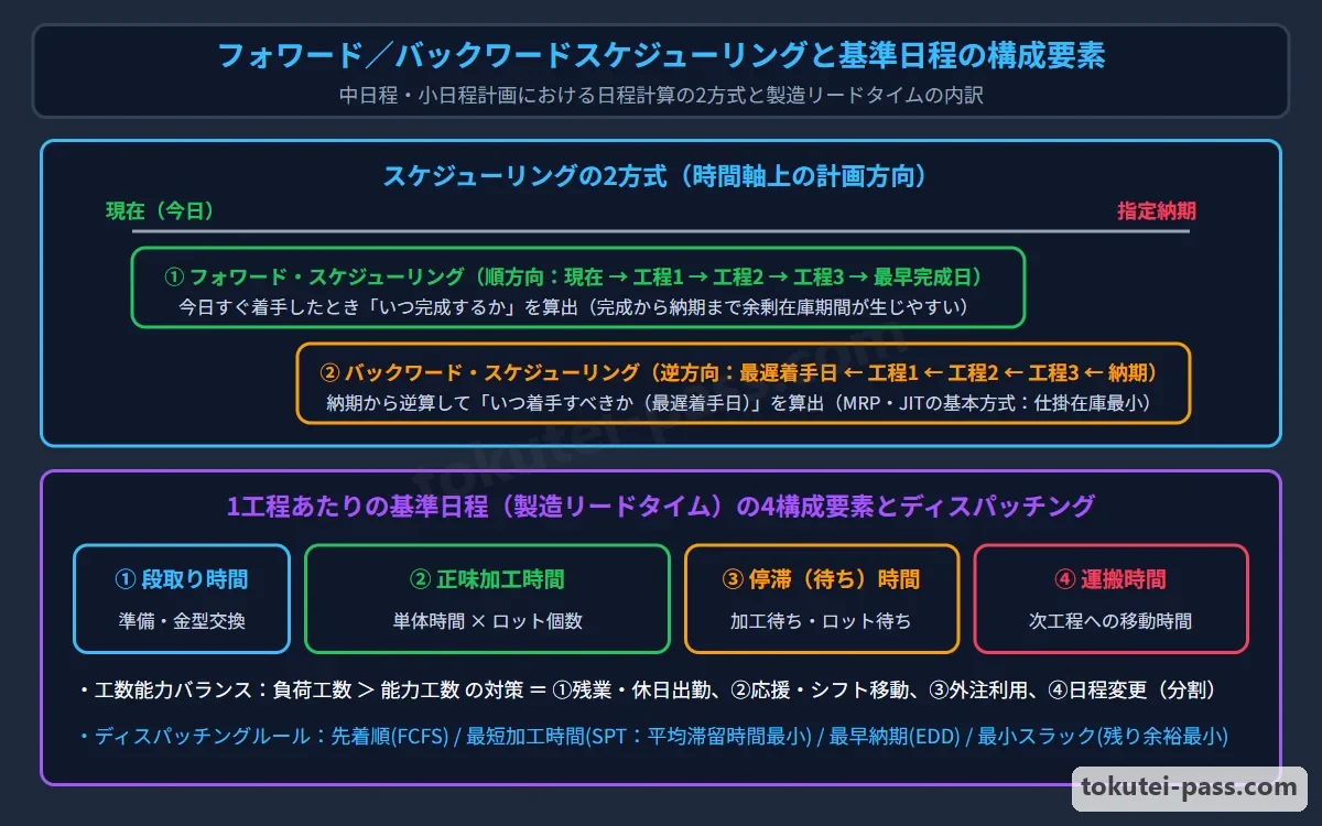
日程計画の立て方には2つの方式があります。仕事の着手可能日(現在)を起点に第1工程から順番に前向きに積み上げて完成予定日を求める「フォワード・スケジューリング」と、顧客の指定納期を起点に最終工程から逆算して各工程の着手日を求める「バックワード・スケジューリング」です。
There are two scheduling methods: Forward Scheduling starts from the earliest available start date (present) and adds process times forward sequentially from Process 1 to find the expected completion date; Backward Scheduling starts from the customer's specified due date and calculates backward from the final process to find the latest start date for each process.
また各工程を通過するのに要する標準的な時間である「基準日程(製造リードタイム)」は、①「加工時間(段取り時間+正味加工時間)」、②「検査時間」、③「運搬時間」、④「停滞時間(工程間の余裕・待ち時間)」の4要素の合計で構成されます。
The Standard schedule (manufacturing lead time)—the standard time required to pass through each process—consists of the sum of four elements: (1) Processing time (setup time + net machining time), (2) Inspection time, (3) Transport time, and (4) Waiting / delay time (inter-process allowance and queue time).
現場で複数の仕事(ジョブ)が待っているとき、どの仕事から先に機械へ投入するかを決める優先規則を「ディスパッチングルール(差立て規則)」と呼びます。
When multiple jobs are waiting on the shop floor, the priority rule deciding which job to load onto a machine first is called a Dispatching Rule.
代表的なルールには、①到着順に処理する「先着順(FCFS)」、②加工時間が最も短い仕事を優先し平均滞留時間を最小にする「最短加工時間ルール(SPT)」、③納期が最も早い仕事を優先する「最早納期ルール(D.Date/EDD)」、④「スラック(=残り持ち時間 - 残り加工時間)」が最小の「最小スラックルール」があります。
Representative rules include: (1) First-Come, First-Served (FCFS) processing in arrival order; (2) Shortest Processing Time (SPT) prioritizing the job with the shortest processing time to minimize mean flow time; (3) Earliest Due Date (D.Date / EDD) prioritizing the job with the earliest due date; and (4) Minimum Slack rule prioritizing the job with the smallest slack (= Remaining time until due date - Remaining processing time).
Key points
- フォワード方式=着手日から順方向に計算し最短完成日を求める/バックワード方式=納期から逆算し最遅着手日を求める(JITやMRPの基本)。
Forward scheduling = Calculates forward from start date to find earliest completion date / Backward scheduling = Calculates backward from due date to find latest start date (basis of JIT and MRP). - 基準日程の4構成要素:①加工時間(段取り+本作業)、②検査時間、③運搬時間、④停滞(余裕)時間。
Four elements of standard schedule: (1) Processing time (setup + main operation), (2) Inspection time, (3) Transport time, (4) Waiting (allowance) time. - 主要ディスパッチングルール:FCFS(先着順)・SPT(最短加工時間優先)・D.Date(最早納期優先)・最小スラック(残り余裕時間が最小のものを優先)。
Major dispatching rules: FCFS (first-come, first-served), SPT (shortest processing time), D.Date (earliest due date), Minimum Slack (smallest remaining margin time). - 【例】現在時刻0日・仕事A(納期10日後・残り加工時間7日)と仕事B(納期8日後・残り加工時間3日) → Aのスラック=10-7=3日、Bのスラック=8-3=5日。最早納期ルールならB優先、最小スラックルールならA優先
Example: At current time Day 0, Job A (due in 10 days, remaining processing time 7 days) and Job B (due in 8 days, remaining processing time 3 days) → A's slack = 10 - 7 = 3 days, B's slack = 8 - 3 = 5 days. Earliest Due Date rule prioritizes B; Minimum Slack rule prioritizes A
| Word | Meaning |
|---|---|
| フォワード・スケジューリングとバックワード・スケジューリング | Forward Scheduling and Backward Scheduling |
| 基準日程の4要素(加工・検査・運搬・停滞時間) | Four elements of standard schedule (Processing, Inspection, Transport, Waiting time) |
| ディスパッチングルール(FCFS・SPT・最早納期・最小スラック) | Dispatching rules (FCFS, SPT, Earliest Due Date, Minimum Slack) |
6. 部品表(BOM:ストラクチャ型とサマリー型)とMRP(有効在庫量・正味所要量計算)
6. Bill of Materials (BOM: Structure vs Summary Type) and MRP (Available Inventory & Net Requirements Calculation)
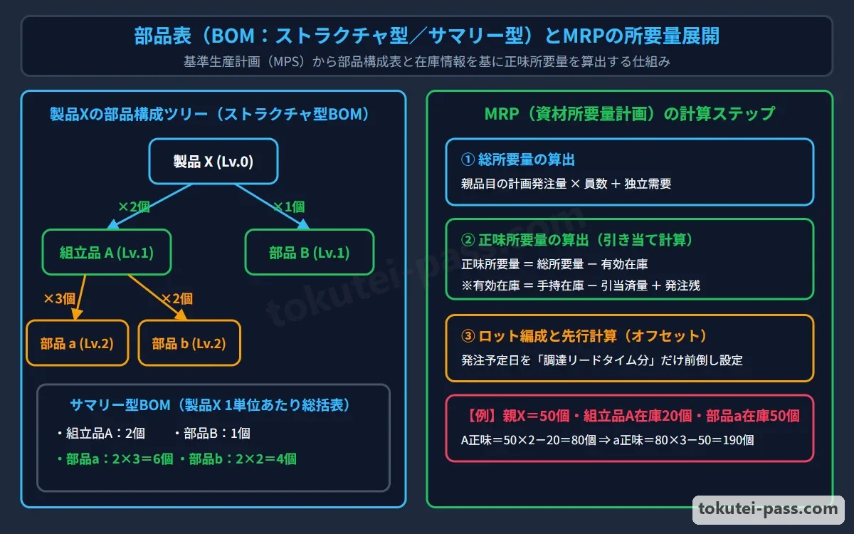
製品1単位を造るのにどの部品・原材料がいくつ必要かを示す「部品表(BOM:Bill of Materials)」には、組立の親子階層構造を1段階ずつそのまま表す「ストラクチャ型(構造型)部品表」と、階層に関係なく製品1個に使われる全部品の合計数量を一覧にした「サマリー型(集計型)部品表」があります。
A Bill of Materials (BOM) showing which parts and raw materials and how many are needed to build one unit of a product has two types: a Structure BOM (indented/single-level BOM) that represents the parent-child assembly hierarchy level by level, and a Summary BOM that lists the total quantity of every part used in one product regardless of hierarchy level.
「MRP(Material Requirements Planning:資材所要量計画)」は、基準生産計画(MPS)とストラクチャ型BOMと在庫情報を用いて、「どの部品が・いつ・何個必要か」を自動計算する仕組みです。まず親品目の生産数に部品構成員数を掛け合わせて「総所要量」を求めます。
MRP (Material Requirements Planning) uses the Master Production Schedule (MPS), Structure BOM, and inventory records to automatically calculate which parts are needed, when, and in what quantity. First, parent production quantities are multiplied by component usage quantities per parent to find Gross Requirements.
次に、現在倉庫にある「手持在庫量」に、すでに発注済みでこれから届く「入庫予定量(注文残)」を足し、他用途に予約済みの「引当済量」や維持すべき「安全在庫量」を引いて、実質的に使える「有効在庫量」を算出します。
Next, Scheduled Receipts (open purchase orders already placed and due to arrive) are added to On-Hand Inventory currently in the warehouse, and Allocated Quantities (reserved for other uses) and required Safety Stock are subtracted to calculate Available Inventory.
そして「総所要量」から「有効在庫量」を差し引いて、真に不足して手配が必要な「正味所要量」を求め、これをロットまとめした上で調達リードタイムだけ前倒し(先行)した日に発注・製造着手を行います。
Then, Available Inventory is subtracted from Gross Requirements to determine Net Requirements (the true shortage that must be procured), which are grouped into lots and ordered or released for manufacturing offset earlier by the procurement lead time.
Key points
- ストラクチャ型BOM=製品・ユニット・部品の親子階層関係を表現(設計変更やMRP展開に適する)/サマリー型BOM=製品1単位あたりの部品総使用数を集計。
Structure BOM = Represents parent-child hierarchical relationships of products, units, and parts (suited for design changes and MRP explosion) / Summary BOM = Totals overall part usage per unit of product. - 有効在庫量 = 手持在庫量 + 入庫予定量(発注残) - 引当済量(および安全在庫量)。
Available Inventory = On-hand inventory + Scheduled receipts (open orders) - Allocated quantity (and safety stock). - 正味所要量 = 総所要量 - 有効在庫量(複数の親ユニットで使われる共通部品は、すべて足し合わせて総所要量を出す)。
Net Requirements = Gross requirements - Available inventory (for common parts used in multiple parent units, sum all requirements to get gross requirements). - 【例】製品Xを100個生産・X1個にユニットAが2個と部品aが1個必要・さらにA1個に部品aが3個必要 → 部品aの総所要量=100×(2×3+1)=700個。手持在庫150個・入庫予定80個・引当済30個なら有効在庫=150+80-30=200個、正味所要量=700-200=500個
Example: Produce 100 units of Product X; 1 X requires 2 Unit As and 1 Part a; 1 Unit A requires 3 Part as → Gross requirement for Part a = 100 × (2 × 3 + 1) = 700 units. With on-hand inventory 150, scheduled receipts 80, and allocated 30, available inventory = 150 + 80 - 30 = 200 units, and net requirement = 700 - 200 = 500 units
| Word | Meaning |
|---|---|
| ストラクチャ型部品表とサマリー型部品表(BOM) | Structure BOM and Summary BOM (Bill of Materials) |
| MRP(資材所要量計画)と総所要量 | MRP (Material Requirements Planning) and Gross requirements |
| 有効在庫量と正味所要量・リードタイム計算 | Available inventory, Net requirements, and Lead-time offsetting |
7. 資材・在庫管理の基礎(常備品と非常備品・定量発注方式と定期発注方式)
7. Basics of Inventory Control (Stock vs Non-Stock Items, Fixed-Order-Quantity vs Periodic-Review Systems)
工場で扱う資材は、多くの製品に共通して反復使用されるため常時一定量を倉庫に在庫しておく「常備品(標準部品・汎用材料等)」と、特定の注文製品にしか使わないため生産計画や受注の都度必要分だけ手配する「非常備品(専用部品等)」に分かれます。
Materials handled in factories are divided into Stock items (standard parts, general materials, etc., kept in constant inventory because they are used repeatedly across many products) and Non-stock / special-order items (dedicated parts, etc., procured only in the required amount each time a production plan or customer order occurs).
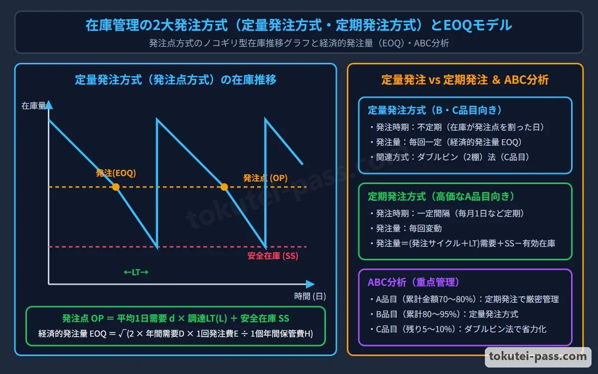
常備品の代表的な補充方式が「定量発注方式(発注点方式)」と「定期発注方式」です。「定量発注方式」は、在庫量があらかじめ定めた「発注点」まで減った時点で、毎回「決まった一定量(経済的発注量など)」を発注する方式です。
The two representative replenishment systems for stock items are the Fixed-Order-Quantity system (Reorder Point system) and the Periodic-Review (Fixed-Interval) system. In the Fixed-Order-Quantity system, whenever inventory drops to a predetermined Reorder Point, a fixed quantity (such as the Economic Order Quantity) is ordered.
定量発注方式は発注時期が不定期で発注量が一定であり、事務手続きが簡単なため単価が安く需要が安定したB・C品目に適します。なお在庫を2つの箱に分け、1箱目が空になった時点で発注する「ダブルビン法(2箱法)」は定量発注の簡便な応用です。
The Fixed-Order-Quantity system has irregular order timing and a fixed order size; because administration is simple, it suits low-unit-cost B and C items with stable demand. The Two-Bin system (Double-bin method)—dividing stock into two bins and reordering when the first bin empties—is a simple application of fixed-quantity ordering.
一方、「定期発注方式」は、毎月1日や毎週月曜日など「決まった発注間隔(発注サイクル)」ごとに需要予測と現在在庫を調べ、毎回異なる必要量を計算して発注する方式であり、単価が高く厳密に在庫圧縮したい重要なA品目に適します。
Conversely, the Periodic-Review system checks demand forecasts and current stock at fixed order intervals (order cycles, e.g., the 1st of every month or every Monday) and calculates a varying required order quantity each time; it suits expensive, critical A items requiring tight inventory reduction.
Key points
- 常備品=反復使用するため常時在庫を持つ資材/非常備品=受注や生産計画の都度、必要量のみを手配する資材。
Stock items = Materials constantly held in inventory for repeated use / Non-stock items = Materials ordered only in required quantities per customer order or production plan. - 定量発注方式=「発注時期は不定期・発注量は一定」(在庫が発注点に達したら一定量を発注、B・C品目向き、ダブルビン法もこの一種)。
Fixed-Order-Quantity system = Irregular order timing, fixed order quantity (orders a fixed amount when stock hits the reorder point; suits B & C items; includes the two-bin method). - 定期発注方式=「発注時期は一定・発注量は毎回変動」(高価で需要変動があるA品目向き)。
Periodic-Review system = Fixed order timing, varying order quantity each time (suits expensive A items with demand fluctuations). - 【例】定期発注方式で発注サイクル30日・調達リードタイム10日・期間中(40日間)の予想需要量800個・安全在庫100個・現在の手持在庫180個・注文残120個 → 今回の発注量=800+100-(180+120)=600個
Example: In a periodic-review system with order cycle 30 days, procurement lead time 10 days, forecast demand during the 40-day period = 800 units, safety stock 100 units, current on-hand stock 180 units, open orders 120 units → Order quantity this time = 800 + 100 - (180 + 120) = 600 units
| Word | Meaning |
|---|---|
| 常備品と非常備品・ABC分析 | Stock items, Non-stock items, and ABC Analysis |
| 定量発注方式(発注点方式・ダブルビン法) | Fixed-Order-Quantity system (Reorder point system / Two-bin method) |
| 定期発注方式(発注サイクル方式) | Periodic-Review system (Order-cycle system) |
8. 発注点・平均在庫量・経済的発注量(EOQ)・安全在庫量の計算公式
8. Formulas for Reorder Point, Average Inventory, Economic Order Quantity (EOQ), and Safety Stock
定量発注方式における「発注点」は、発注してから品物が納入されるまでの「調達期間(リードタイム)中の推定消費量」に「安全在庫量」を加えたものであり、「発注点 = 1日平均需要量 × 調達リードタイム(日) + 安全在庫量」で計算します。
The Reorder Point in a fixed-order-quantity system equals estimated consumption during the procurement lead time (from order placement to delivery) plus safety stock: Reorder Point = Average daily demand × Procurement lead time (days) + Safety stock.
また1回の発注量をQとすると、在庫は「安全在庫+Q」と「安全在庫」の間をのこぎり歯状に増減するため、「平均在庫量 = 1回の発注量Q ÷ 2 + 安全在庫量」となります。
If the order quantity per order is Q, inventory fluctuates in a sawtooth pattern between (Safety stock + Q) and Safety stock, so Average Inventory = Order quantity Q ÷ 2 + Safety stock.
年間の「発注費用」と「在庫保管費用」の合計(総費用)が最小となる1回あたりの最適発注量を「経済的発注量(EOQ)」と呼び、「EOQ = √(2 × 年間需要量D × 1回発注費S ÷ 1個あたり年間保管費H)」で求めます(H = 購入単価P × 年間保管費率i)。
The optimal order quantity per order that minimizes the sum of annual ordering cost and annual inventory holding cost (total cost) is the Economic Order Quantity (EOQ), calculated as: EOQ = √(2 × Annual demand D × Ordering cost per order S ÷ Annual holding cost per unit H), where H = Unit purchase price P × Annual holding cost rate i.
さらに需要変動による品切れを防ぐ「安全在庫量」は、「安全係数α × 1日(または単位期間)の需要の標準偏差σ × √(調達リードタイムL + 発注サイクルT)」で求めます(定量発注ではT=0)。試験では「許容欠品率(品切れ率)5%のとき安全係数α = 1.65」が頻出です。
Furthermore, Safety Stock to prevent stockouts from demand fluctuations is calculated as: Safety factor α × Standard deviation of daily (or unit-period) demand σ × √(Procurement lead time L + Order cycle T) (where T = 0 in fixed-order-quantity systems). In exams, 'allowable stockout rate of 5% gives safety factor α = 1.65' appears frequently.
Key points
- 発注点 = 1日平均需要量 × 調達リードタイム + 安全在庫量/平均在庫量 = 発注量 ÷ 2 + 安全在庫量。
Reorder Point = Average daily demand × Procurement lead time + Safety stock / Average Inventory = Order quantity ÷ 2 + Safety stock. - 経済的発注量(EOQ)= √(2 × 年間需要量 × 1回発注費 ÷ (単価 × 年間保管費率))(発注費用と保管費用が等しくなる点)。
Economic Order Quantity (EOQ) = √(2 × Annual demand × Ordering cost per order ÷ (Unit price × Annual holding cost rate)) (the point where ordering cost equals holding cost). - 安全在庫量 = 安全係数(欠品率5%なら1.65) × 需要標準偏差σ × √(調達期間L + 発注間隔T)(※定量発注はT=0)。
Safety Stock = Safety factor (1.65 for 5% stockout rate) × Demand standard deviation σ × √(Lead time L + Order interval T) (T = 0 for fixed-order-quantity system). - 【例】1日平均需要50個・標準偏差10個・調達期間4日・許容欠品率5%(係数1.65)の定量発注 → 安全在庫=1.65×10×√4=33個、発注点=50×4+33=233個。また年需要12,000個・1回発注費1,500円・単価500円・年保管費率20%(保管費100円/個)ならEOQ=√(2×12,000×1,500÷100)=√360,000=600個
Example: Fixed-quantity ordering with average daily demand 50 units, standard deviation 10 units, lead time 4 days, allowable stockout rate 5% (factor 1.65) → Safety stock = 1.65 × 10 × √4 = 33 units, Reorder point = 50 × 4 + 33 = 233 units. Also, if annual demand is 12,000 units, ordering cost 1,500 yen/order, unit price 500 yen, annual holding rate 20% (holding cost 100 yen/unit), EOQ = √(2 × 12,000 × 1,500 ÷ 100) = √360,000 = 600 units
| Word | Meaning |
|---|---|
| 発注点と平均在庫量 | Reorder Point and Average Inventory |
| 経済的発注量(EOQ:Economic Order Quantity) | Economic Order Quantity (EOQ) |
| 安全在庫量と許容欠品率5%(安全係数1.65) | Safety Stock and 5% Allowable Stockout Rate (Safety factor 1.65) |
試験によく出るポイントと覚え方
Frequent Exam Points and How to Remember Them
第3章(問9〜問18)は専門知識25問のうち10問を占める最重要章であり、計算問題が集中します。まず「生産計画の3分野(手順・工数・日程)」と「生産統制の5分野(手配・ディスパッチング・進捗・現品・余力)」の分類と帳票対応を確実に区別しましょう。
Chapter 3 (Questions 9 to 18) accounts for 10 of the 25 specialized questions—the most heavily weighted chapter, packed with calculation problems. First, clearly distinguish the 3 areas of Production Planning (routing, workload, scheduling) and 5 areas of Production Control (order release, dispatching, progress, physical WIP, capacity) and their corresponding forms.
工数計画の計算では、不適合品率rが与えられたときに負荷工数を「適合品率(1-r)で割る」ことが最大のポイントです。また人的生産能力(人員・時間・出勤率・稼働率・能率の積)と機械生産能力の式も頻出です。
In workload calculations, when a non-conforming (defect) rate r is given, the most critical point is dividing the required workload by the conforming rate (1 - r). Formulas for human production capacity (product of workers, hours, attendance rate, operating ratio, efficiency) and machine capacity also appear frequently.
日程計画とMRPでは、基準日程の4要素(加工・検査・運搬・停滞)、ディスパッチングルールの「最小スラック(残り持ち時間から残り加工時間を引いた余裕が最小)」、BOMツリーからの「総所要量」と「有効在庫量(手持+入庫予定-引当)」「正味所要量」の計算が毎回出題されます。
In scheduling and MRP, the 4 elements of standard schedule (processing, inspection, transport, waiting), the Minimum Slack dispatching rule (remaining time to due date minus remaining processing time), and calculating Gross Requirements from a BOM tree along with Available Inventory (on-hand + scheduled receipts - allocated) and Net Requirements are tested on every exam.
在庫管理では「定量発注(発注点で一定量を発注・BC品目)」と「定期発注(一定期間ごとに発注量を計算・A品目)」の対比、および発注点・平均在庫量・EOQ・安全在庫量(許容欠品率5%で安全係数1.65)の4公式を必ずマスターしてください。
In inventory control, master the contrast between Fixed-Order-Quantity (fixed amount at reorder point, B/C items) and Periodic-Review (calculated amount at fixed intervals, A items), plus the 4 major formulas: Reorder Point, Average Inventory, EOQ, and Safety Stock (safety factor 1.65 at 5% allowable stockout rate).
Key points
- 3計画(手順・工数・日程)と5統制(手配・差立て・進捗・現品・余力)、および需要変動への3つの緩衝(モノ・能力・時間)。
3 Plans (routing, workload, scheduling) & 5 Controls (order release, dispatching, progress, physical WIP, capacity), plus 3 buffers against demand change (goods, capacity, time). - 不適合品があるときの負荷工数は「適合品率(1-不適合品率)で割る」。MRPでは「正味所要量=総所要量-(手持在庫+入庫予定-引当済)」。
When defects exist, divide workload by the conforming rate (1 - defect rate). In MRP: Net requirements = Gross requirements - (On-hand + Scheduled receipts - Allocated). - 在庫4大公式:①発注点、②平均在庫量、③EOQ(経済的発注量)、④安全在庫量(欠品率5%の安全係数=1.65)。
Four major inventory formulas: (1) Reorder Point, (2) Average Inventory, (3) EOQ (Economic Order Quantity), (4) Safety Stock (safety factor = 1.65 for 5% stockout rate).
| Word | Meaning |
|---|---|
| 3計画・5統制と3つの緩衝 | 3 Plans, 5 Controls, and 3 Buffers |
| 負荷工数・最小スラック・正味所要量 | Workload, Minimum Slack, and Net Requirements |
| 発注点・EOQ・安全在庫量の公式 | Formulas for Reorder Point, EOQ, and Safety Stock |
Production Planning, Process & Inventory Control (MRP)
Practice this chapter in the appOfficial references
- 中央職業能力開発協会(JAVADA) ビジネス・キャリア検定試験 3級 生産管理プランニング 試験範囲 — https://www.javada.or.jp/jigyou/gino/business/subject.html
- 中央職業能力開発協会 編『ビジネス・キャリア検定試験 標準テキスト【専門知識】生産管理プランニング 3級〔第4版〕』 — https://www.javada.or.jp/jigyou/gino/business/text.html